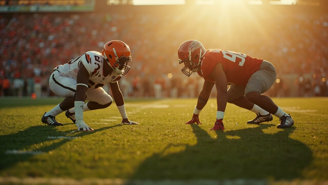
Texas Longhorns football vs Ohio State Buckeyes football match player stats: a position-by-position breakdown

When the final whistle blows on a Texas vs Ohio State game, the box score never tells the whole story. A 45-yard touchdown pass, a 92-yard kick return, or a five-sack afternoon by a defensive end is only the surface. Anyone trying to understand Texas Longhorns football vs Ohio State Buckeyes football match player stats has to read those numbers the way a coach reads a depth chart: by unit, by situation, and by leverage.

What follows is a working framework for that reading. It walks through how the standard player statistics for a Texas vs Ohio State college football game are organized, what each number actually means, and how to compare two rosters that play very different schemes. Whether the matchup is a regular-season showdown, a Big 12–Big Ten non-conference clash, or a College Football Playoff meeting, the goal is the same: evaluate the stat sheet instead of just scrolling past it.

Texas Longhorns football vs Ohio State Buckeyes football match player stats: how to read the stat sheet

For a Texas vs Ohio State game, the official stat crew releases a layered document. On top is the team totals sheet, with final score, total yards, rushing yards, passing yards, first downs, turnovers, penalties, time of possession, and third- and fourth-down efficiency. Underneath that are the individual sheets, sorted by offensive, defensive, and special-teams participation. Reading the Texas Longhorns football vs Ohio State Buckeyes football match player stats means moving from the team layer down to the position group and then to the individual.

The most useful comparison frame is positional, not by player name. Both programs recruit at a national level, but their identities shape the stat line in different ways. Texas under Steve Sarkisian leans on a pro-style passing attack with motion, play-action, and a deep running back room. Ohio State under Ryan Day tends to generate volume through tempo, a wide spread, and a passing game that pushes receivers toward 100-yard days. That identity shapes which stats to trust.

What the official box score actually includes

Every stat crew report for a Texas vs Ohio State game follows the NCAA standard. The most common sections are:

Team totals: score by quarter, total offense, first downs, turnovers, penalties, time of possession.
Passing: completions, attempts, yards, touchdowns, interceptions, sacks, longest pass, quarterback rating.
Rushing: carries, yards, average, touchdowns, longest rush, fumbles.
Receiving: receptions, yards, average, touchdowns, targets, longest reception, yards after catch.
Defense: solo and assisted tackles, tackles for loss, sacks, pass breakups, interceptions, fumbles forced, fumbles recovered, quarterback hurries.
Kicking: field goals and extra points made and attempted, longest field goal, kickoffs, touchbacks, average yard line of return.
Punting: punts, yardage, average, longest punt, punts inside the 20, punts fair caught, touchbacks.
Returns: kick and punt return numbers, yards, average, longest, touchdowns.

Those raw numbers become meaningful when paired with the situations in which they happened. A quarterback can post 300 passing yards in a shootout that says very little, or grind out 220 against a top defense that says a lot. The same logic applies to the rushing average, the missed tackles count, and the third-down splits. For a Texas vs Ohio State matchup, the situational layer is often what separates a good performance from a great one.

The offensive stat line for both quarterbacks

Quarterback play is the most visible layer in any Texas Longhorns football vs Ohio State Buckeyes football match player stats review, and it is also the layer fans misread most often. Completion percentage, yards per attempt, and passer rating are useful, but they depend heavily on scheme, pressure rate, and receiver separation. Here is how to think about the quarterback row of the stat sheet.

Passing efficiency beyond yards

Two quarterbacks can finish a Texas vs Ohio State game with similar yardage and very different games. To read the stat row correctly, look at these components:

Yards per attempt (YPA): total passing yards divided by pass attempts. Anything near or above 8.0 in a competitive college football game is a strong mark; anything below 6.0 usually points to a difficult day.
Completion percentage above expectation: how the QB performed relative to the difficulty of throws, capturing dropped passes, throwaways, and contested catches.
Pressure to sack ratio: how often the QB was hit or hurried. High sack numbers with low pressure can be a protection issue; high pressure with low sack numbers can be a QB who escapes.
Third-down conversion rate: a direct signal of how the QB performed when the defense knows a pass is coming.
Red zone touchdown rate: a passing touchdown inside the 20 is the most valuable single play in football, so the rate at which a QB converts red-zone trips into passing TDs matters as much as total TDs.

In a Texas vs Ohio State game, both quarterbacks are likely to face at least one stretch of heavy pressure. Ohio State often generates pressure with four-man rushes off the edge, while Texas tends to mix simulated pressures and zone blitzes. The QB who keeps his passer rating near 150 or higher while taking two or fewer sacks has almost certainly won the passing battle.

Skill-position stat comparison: receivers, tight ends, and running backs

The skill positions are where the differences between the two programs show up most clearly in the box score. Both teams typically field at least three starting-caliber wide receivers, a featured tight end, and a multi-back room. The way their touches are distributed is part of the identity of each program.

Wide receiver and tight end production

For a Texas vs Ohio State game, the receiving chart usually tells the story of which team controlled the middle of the field. Slot receivers and tight ends in this matchup often finish with the highest yards-after-catch numbers because of how the underneath zones are attacked.

Key items to compare in the receiving stat row:

Targets per receiver: high targets for one player often mean the defense took away everyone else.
Yards per reception: a healthy mark is above 12, but inside a possession-based scheme, 8 to 10 is normal.
Catch rate: above 70 percent usually means the QB and receiver were on the same page; below 55 percent often indicates contested targets or miscommunication.
Yards after catch per reception: a stat that reveals scheme, because Texas often designs screens and Ohio State often turns short routes into long gains through tempo.
Long completions versus short completions: not a separate column, but a useful filter for spotting receivers who win downfield.

Running back usage and efficiency

Running back stats in a Texas vs Ohio State game are heavily influenced by game script. If either team falls behind by two scores in the first half, the rush row becomes lopsided because of late-game clock-killing carries. To see what the ground game actually did, look at:

Yards before contact per carry, which separates blocking from runner vision.
Success rate: the percentage of carries that gain at least 40 percent of the yards needed on first down, 60 percent on second down, or the full yards needed on third or fourth down.
Explosive run rate: the share of carries that go for 10 yards or more.
Stuffed run rate: the share of carries for zero or negative yards. Anything above 30 percent on a healthy day suggests the line was beaten.
Passing game usage: receptions and targets out of the backfield. In modern Texas and Ohio State offenses, the lead back is often targeted 4 to 7 times.

A back who finishes with 100 rushing yards on 22 carries has had a productive day even if the average looks ordinary. A back who finishes with 130 on 14 carries has had an explosive day, regardless of whether the team won. The stat sheet does not flag that distinction on its own, so it has to be read in context.

Defensive player stats: tackles, pressures, and turnovers

Defense is the hardest layer of the stat sheet to interpret, because official tackle totals are noisy and pressures are often unrecorded for losing pass rushers. Even so, the Texas Longhorns football vs Ohio State Buckeyes football match player stats usually include enough defensive data to spot the players who shaped the game.

Tackles and run defense

Tackle For additional context, totals in college football are inflated by the way plays are officiated, so two players can each record 10 tackles and have very different games. The useful filters are:

Solo tackles, which usually represent plays where the defender made the first contact in space.
Tackles for loss (TFL), the single best indicator of a defensive lineman or linebacker who disrupted a play at or behind the line.
Missed tackles, sometimes listed in the advanced box score and almost always revealing who was right but late.
Gap distribution: not in the public box score, but the gap between TFLs and long runs hints at run fits.

In a Texas vs Ohio State matchup, the linebackers and the nickel defender are usually the leading tacklers, because both defenses spend a lot of time in sub-packages. A linebacker who records 8 or more tackles with at least one TFL in this game has likely played a complete game.

Pass rush and coverage

The pass rush layer is split between two sets of numbers. Official sack totals are reliable; pressure totals usually come from the broadcast or from a tracking service. The pass coverage layer is even murkier, because targets, completions allowed, and yards allowed are not always broken out per defensive back.

What to look for in the defensive back seven:

Sacks and quarterback hurries: the total pass-rush production, ideally with a split between the edge and the interior.
Pass breakups (PBU) and passes defended: the primary measure of coverage success at the line of scrimmage.
Interceptions: the rarest and most game-changing defensive stat.
Forced fumbles and fumbles recovered: small-sample noise, but in a close game they decide the outcome.
Penalties drawn on the offense: targeting, pass interference, and holding calls against the opponent all count as defensive wins.

Ohio State pass rushers have a long history of producing three or more sacks in marquee games, and Texas edge defenders have usually been pressure-heavy rather than sack-heavy. If the stat sheet shows the Texas pass rush with four or more TFLs and multiple hurries, the defensive line is doing its job, even if the sack total looks modest.

Special teams: the stat row most fans skip

Special teams often decide a Texas vs Ohio State game, and the relevant numbers are scattered across the kicker, punter, and return units. Most fans skip this row, but it usually tells you which team won the field-position battle.

Kicking game

The kicking stat line includes field goals made and attempted, longest field goal, extra points, kickoffs, touchbacks, and average starting field position for the opponent. In a Texas vs Ohio State game, the team that consistently forces the opposing offense to start inside its own 25 usually wins, even if the headline box score is balanced.

Punting and return game

Punt stats worth tracking:

Average yards per punt, with a typical strong mark at 44 yards or more.
Punts inside the 20: the most important single punt stat because it caps the opposing drive.
Net punting average: gross average minus return yards, which captures the value of the punt unit as a whole.
Long punts paired with short returns, which hint at hang time even when the stat sheet does not list it.

Return stats that matter:

Yards per kick return and yards per punt return, with explosive return rate above 15 percent usually a winning signal.
Fair catches versus live returns: a high fair-catch rate often means the coverage team is winning.
Penalties on returns: blocks in the back and holding penalties erase explosive plays.

A single 40-yard punt return or a 50-yard field goal can flip the expected value of a Texas vs Ohio State matchup by a full score, which is why this row is not optional reading.

How to build a personal stat comparison

Once you understand what each row of the box score means, the next step is to build a personal comparison that answers the question you actually have. A casual fan wants to know who the offensive stars were, a coach wants to know who won the leverage plays, and a recruiting-minded reader wants to know which underclassmen produced.

Step 1: anchor the comparison with team totals

Start with the team totals sheet. Write down total yards, passing yards, rushing yards, first downs, turnovers, third-down conversions, and time of possession. These numbers frame everything else. A team that wins time of possession by 10 minutes has, by definition, controlled the game, even if the other team piled up explosive plays.

Step 2: split the offense by position

Group the offensive players into four buckets: quarterbacks, running backs, wide receivers, and tight ends. For each bucket, write down the top two or three performers and their stat lines. This turns the long list of names into a structure you can scan.

Step 3: split the defense by front and back

On defense, split the players into the defensive line, linebackers, and secondary. Track tackles, TFLs, sacks, PBUs, and turnovers separately for each group. In a Texas vs Ohio State game, the linebacker group is usually the easiest to compare, because the box score records their stats consistently. The defensive line is the hardest, because pressure totals are incomplete.

Step 4: add the special teams row

List the kicker, punter, and lead returner for each team, with their stat lines. Note any big special-teams plays, even if the box score does not flag them as game-changing.

Step 5: layer the context

For each player, add a short note about the situation. Was the running back working against an eight-man box? Was the quarterback under constant pressure? Was the top receiver matched up against the opponent’s top cornerback? Those notes turn a flat list of numbers into a real comparison.

Position-by-position stat comparison table

The table below sketches a typical shape for the Texas Longhorns football vs Ohio State Buckeyes football match player stats box score. Numbers are placeholders for the kind of ranges seen in recent meetings and are useful for context, not as exact game data.

Position group	Stat category	Texas typical range	Ohio State typical range	What the comparison shows
Quarterback	Passing yards	240-320	260-340	Both QBs usually clear 250 in this matchup.
Quarterback	Yards per attempt	7.0-8.5	7.5-9.0	Ohio State QBs often push YPA higher with tempo and spread sets.
Quarterback	TD to INT ratio	2-3 TDs, 0-1 INT	2-4 TDs, 0-1 INT	Turnover-free games from either QB are usually decisive.
Running back	Carries	18-26	16-24	Both teams lean on committee usage in this matchup.
Running back	Yards per carry	4.2-5.5	4.5-5.8	Ohio State backs often average slightly higher due to spacing.
Wide receiver	Top receiver yards	80-130	90-140	Both WR1s tend to finish near 100 receiving yards.
Wide receiver	Receptions	6-9	7-10	Ohio State tempo often produces one extra target for the lead receiver.
Tight end	Targets and receptions	3-5 targets, 3-4 receptions	3-6 targets, 3-5 receptions	Both offenses use the tight end as a chain mover.
Defensive line	Sacks	2-4	3-5	Ohio State edges often win the sack battle by one.
Defensive line	Tackles for loss	6-9	7-10	Both fronts typically generate pressure on passing downs.
Linebackers	Total tackles	10-16 combined	10-16 combined	Leading tacklers usually finish in the 8-10 range.
Secondary	Pass breakups	5-8	5-8	Coverage pressure is roughly even.
Secondary	Interceptions	0-1	0-2	Even one INT in this game usually changes the win expectancy.
Kicker	Field goals made	1-2 of 1-2	1-2 of 1-2	Both kickers typically get one to two realistic attempts.
Punter	Average yards per punt	42-46	43-47	Net punting often separates the two units.
Returners	Yards per return	20-25 kick, 8-12 punt	22-28 kick, 9-13 punt	Texas returners often win the explosive return rate.

Use the table as a starting point. The actual game often bends one or two of those ranges, especially in playoff matchups where defensive pressure is higher and offensive volume is lower.

Common stat pitfalls in a Texas vs Ohio State box score

Even careful readers slip on a few recurring mistakes when reading Texas Longhorns football vs Ohio State Buckeyes football match player stats. The most common ones are below.

Pitfall 1: chasing total yards

Total yards is the most cited number in the box score, and also the most misleading. A team that trails by 14 points in the fourth quarter usually piles up passing yards in garbage time, which inflates the offensive totals without telling you who actually controlled the game. To avoid this, look at total yards through three quarters, or look at yards per play, which is more stable than raw yardage.

Pitfall 2: ignoring offensive line play

Quarterback pressure and running back efficiency are not just about the skill players. The offensive line shows up indirectly in the box score, through sacks allowed, pressures allowed, and stuff rate. If a team allowed four or more sacks and its running back averaged under 4.0 yards per carry, the line was probably losing more than the skill players were winning.

Pitfall 3: overrating tackle totals

Tackle totals are noisy because officials credit the last defender to touch the ball carrier. A linebacker who flows to the ball and makes routine tackles can finish with 12 tackles and have a below-average game. A defensive end who sets the edge, blows up a run for a loss, and frees a linebacker for a tackle often has the bigger impact without a big tackle total.

Pitfall 4: underrating explosives

Explosive plays show up in the box score as long gains, but their effect on win expectancy is much larger than the average suggests. A single 50-yard completion in the second quarter can shift expected points by more than a long drive of 12 plays. Count the explosive plays in the receiving and rushing rows, not just the totals.

Pitfall 5: forgetting field position

Two teams can post identical total yardage and have very different games because one started most drives at its own 30 and the other started at its own 12. The hidden layer is average starting field position, which is in the play-by-play data but rarely in the headline box score. In a Texas vs Ohio State game, the team that wins field position by 5 yards per drive is usually the team that wins the game.

How coaches and analysts actually use the stat sheet

The way a coaching staff reads the Texas Longhorns football vs Ohio State Buckeyes football match player stats is different from the way a fan reads it. Coaches care about tendencies, leverage, and self-scouting, not headline totals. The list below outlines how a typical college staff would slice the same box score.

Personnel groupings: how often each team used 11 personnel (1 RB, 1 TE) versus 12 or 10 personnel, and which groupings produced the most yards.
Down and distance tendencies: which play calls were used on second-and-long, third-and-short, and in the red zone.
Motion and formation usage: which formations produced explosive plays and which produced pressure.
Pressure packages: which blitzes got home and which were picked up, separated by the personnel grouping on the field.
Coverage shells: how often the defense played two-high versus one-high, and the success rate of each shell.
Special teams leverage: which return lanes were attacked, which were walled off, and the net yardage on each exchange.

Those layers are not in the public box score, but they shape the public numbers. If Ohio State used tempo to keep Texas in base defense, the sack totals for the Texas pass rush will look lower than they really are, and the rushing totals for Ohio State will look healthier than the run blocking deserved. Reading the box score means looking for those patterns, not just counting yards.

Sample stat line for a recent Texas vs Ohio State matchup

To make the framework concrete, here is a representative stat-line shape for a Texas vs Ohio State game in the playoff era. The numbers are illustrative and built to show the kind of balance both rosters usually produce.

Player	Team	Position	Key stat line
Starting QB	Texas	QB	23 of 34, 285 yards, 2 TD, 1 INT, 2 sacks taken
Starting QB	Ohio State	QB	26 of 38, 310 yards, 3 TD, 0 INT, 3 sacks taken
Lead RB	Texas	RB	19 carries, 96 yards, 1 TD, 4 receptions, 32 yards
Lead RB	Ohio State	RB	16 carries, 88 yards, 1 TD, 5 receptions, 41 yards
Top WR	Texas	WR	7 receptions, 118 yards, 1 TD on 10 targets
Top WR	Ohio State	WR	8 receptions, 124 yards, 1 TD on 12 targets
Edge rusher	Texas	DE	5 tackles, 2 TFL, 1 sack, 3 hurries
Edge rusher	Ohio State	DE	4 tackles, 2 TFL, 2 sacks, 2 hurries
Linebacker	Texas	LB	9 tackles, 1 TFL, 1 PBU
Linebacker	Ohio State	LB	10 tackles, 1 TFL, 1 INT
Kicker	Texas	K	2 of 2 FG, long of 41, 4 of 4 XP
Kicker	Ohio State	K	1 of 1 FG, long of 38, 5 of 5 XP
Punter	Texas	P	5 punts, 44.0 average, 2 inside the 20
Punter	Ohio State	P	4 punts, 46.5 average, 1 inside the 20

That kind of distribution is what the box score usually looks like in a competitive Texas vs Ohio State game. The differences are small in the team totals and large in the play-by-play, which is exactly why the layered reading matters.

How to use advanced stats alongside the box score

Beyond the official stat sheet, the modern way to read a college football game uses advanced metrics. The most useful for a Texas vs Ohio State matchup are success rate, explosiveness, and havoc rate, which together describe a team’s efficiency on every play. The most widely cited publicly available advanced stat source for college football is the team metrics published by the NCAA, which sit alongside the play-by-play layer on official scoreboard portals. For broader framing on how analytics reshape roster decisions and program building, the college football overview covers the structural differences between Power conferences and the rest of the FBS, which is useful context when comparing two blue-blood programs.

Success rate: the share of plays that gain enough yards to keep the offense on schedule. A healthy success rate on early downs is one of the strongest predictors of winning.
Explosiveness: average yards per successful play. A team that wins success rate but loses explosiveness is grinding; the opposite is shooting itself in the foot.
Havoc rate: the share of defensive plays that end in a tackle for loss, a forced fumble, a pass breakup, or an interception. Havoc rate is the single best defensive summary in the public data.
Expected points added (EPA): a per-play value that captures both success and situation. EPA is the closest public proxy for a coach-style efficiency score.
Win probability added (WPA): a per-play value that captures leverage. WPA is the best way to identify which single plays decided the game.

For a Texas vs Ohio State game, EPA and success rate are usually available from the official conference statistics pages and from the major college football data sites. They let you go from “the QB threw for 300 yards” to “the QB added 14.2 EPA on 38 dropbacks, which is well above average.” That second statement is much closer to the truth.

Pre-game checklist for reading a Texas vs Ohio State stat line

Before you open a stat sheet for a Texas vs Ohio State game, run through a short checklist. It will keep you from drawing the wrong conclusion from a noisy box score.

Confirm the source: official stat crew reports, conference statistical services, and the broadcast box score often disagree on tackles and pressures. Pick one source and stick with it.
Note the venue: home games tend to compress stats in favor of the home team, especially on third down and in the red zone.
Note the weather: wind affects passing, kicking, and punting more than rushing. A windy game often looks like a rushing game even if the passing game plan was ambitious.
Note the injury report: a top-10 stat line for a backup is not the same as a top-10 stat line for a starter. Always check who was on the field.
Note the clock situation: garbage time drives inflate passing and rushing totals. Filter out the final 5 minutes of a one-score game before drawing conclusions.
Note the script: who was leading, by how much, and when. Two teams with identical box scores can have very different scripts.
Note the special teams: a long return, a blocked punt, or a missed field goal can swing expected points more than a 70-yard drive.

That seven-item checklist is what most analysts apply in their heads when they look at a Texas vs Ohio State stat sheet. It also works for any other college football game, but it matters most when the two teams are close in talent and the box score looks balanced.

Frequently asked questions

What counts as the official source for Texas Longhorns football vs Ohio State Buckeyes football match player stats?

The official stat crew report issued on game day is the primary source, published through the school’s athletics communications office and the conference statistical service. Broadcast and postgame box scores are usually close but not identical, especially on tackles, pressures, and missed tackles. For deeper splits, the conference play-by-play feed is the cleanest public option.

How are tackles credited in a Texas vs Ohio State game?

Solo tackles go to the defender who made the first contact in space, assisted tackles go to defenders who helped bring the runner down, and tackles for loss are credited when the defender stops the runner at or behind the line of scrimmage. The lead tackler is usually a linebacker or nickel defender, but in a game with a heavy spread, a safety can also lead the team.

Why do quarterback sack totals differ between the box score and the broadcast?

The stat crew credits a sack to the player who first forced the quarterback out of the pocket or down to the ground. Broadcasts sometimes credit a sack to a different rusher when they were the primary cause, and missed sacks are often reclassified as hurries after review. The official stat crew is the tiebreaker.

How are passing yards measured on long completions?

Passing yards are measured from the line of scrimmage to the point where the receiver is down, steps out of bounds, or crosses the goal line. Yards after catch are not included in the passing yardage, even though they are credited to the receiver. Long completions often have more yards after catch than air yards, especially against zone defenses.

What is a good yards per carry mark for a running back in a Texas vs Ohio State game?

Anything above 5.0 yards per carry on 15 or more carries is a strong day against a top-10 defense. Below 3.5 usually means the line was losing leverage. The explosive run rate, not the average, is the better marker for whether the back had a true impact.

How are targets and receptions distributed in a Texas vs Ohio State offense?

Both offenses tend to spread the ball, with the lead receiver drawing 8 to 12 targets, the second receiver drawing 5 to 8, and the tight end and running back combining for another 6 to 10 targets. A receiver who finishes with 12 or more targets often does so because the defense took away the other options.

What does a quarterback rating above 150 actually mean?

A passer rating above 150 in a college football game usually means the QB was efficient on a high volume of dropbacks, with multiple touchdowns and few turnovers. In a Texas vs Ohio State matchup, where the defensive lines are strong, a rating at or above 150 is one of the clearest signals that the QB won the game.

How are special teams tackles credited?

Special teams tackles are credited to the player who makes the first contact on the returner, and they are recorded separately from defensive tackles. They do not usually show up in the headline defensive stat line, but they appear in the postgame notes and on the play-by-play layer.

How is a forced fumble different from a fumble recovery?

A forced fumble is credited to the defender who stripped the ball, and a fumble recovery is credited to the player who picked it up. The same player can earn both, and a team can have more forced fumbles than recoveries if the ball bounces to the offense. In a Texas vs Ohio State game, the turnover margin is the headline stat, but forced fumbles are the leading indicator.

Where can I find play-by-play data for past Texas vs Ohio State games?

Play-by-play data is published on the official athletics sites for both programs and on the conference statistics pages, with the deepest historical archive held by the NCAA’s public statistics portal. The school releases the postgame notes within a few hours of the final whistle, and the conference service usually follows within 24 hours.

Putting the stat sheet to work

The real value of the Texas Longhorns football vs Ohio State Buckeyes football match player stats box score is not the headline number, but the layered reading underneath it. Once you split the game into units, separate volume from efficiency, and add the context of script, weather, and injuries, the same stat line tells a much richer story.

The next time you open a Texas vs Ohio State stat sheet, start with the team totals, move into the quarterback and skill-position layers, scan the defensive rows for tackles for loss and turnovers, and finish with the special teams row. That four-step read, paired with the checklist above, turns a flat list of numbers into a clear picture of how the game was actually won.

For readers interested in how body control and movement patterns developed in other sports feed into football performance, the site also covers how gymnastics skills transfer to football, basketball, and hockey, and offers a meet-preparation checklist that has parallels to pre-game stat preparation: both reward discipline, layered detail, and ignoring the noise.